How Tokens Work

In this post, I want to explore what AI tokens actually are and how they work.

Until now, I have mainly written about how to use AI tools effectively, which tools are gaining popularity, and why. But while putting together my guide to saving tokens, I was reminded of something important: before explaining how to reduce costs, I first needed to explain what tokens are and how they are billed. Yet I had never properly covered that foundation. (As I wrote the cost-saving guide, the explanation of how tokens work grew substantial enough to become a post of its own.)

This post, then, lays the groundwork before we get into cost-saving techniques. We will go through what tokens actually are if they are neither words nor characters (BPE), what form they take when they enter a model (embeddings), why output is more expensive than input (prefill/decode), where inside the Transformer architecture prompt caching gets its cost advantage (KV cache), and why longer contexts become more expensive (the quadratic cost of attention). If you are looking for practical ways to save, continue with How to Save Tokens after this article.

---

Tokens Are Neither Words nor Characters

Let us start with the most fundamental fact: a token is neither a word nor a character. It is a unit in a vocabulary built by compressing character sequences that occur frequently in the model's training data.

Our intuition for asking “How many words are in this sentence?” differs from the way a model splits text. A model groups character combinations that frequently appear together into single units, then segments incoming text according to that vocabulary. As a result, one word may be represented by a single token while another is split into several.

The algorithm used to build this vocabulary is BPE, a common foundation of nearly every modern LLM.

The BPE Algorithm

BPE (Byte Pair Encoding) is an algorithm that grows a vocabulary by repeatedly merging the most frequent pair of adjacent symbols into a new symbol.

Interestingly, it was not originally created for natural language processing. Philip Gage first proposed BPE in 1994 as a data compression technique. The method replaced the most frequently occurring byte pair in a dataset with a single byte not otherwise used in the data, then stored those replacement rules separately in a table.

A research team led by Sennrich at the University of Edinburgh brought the technique to the vocabulary problem in neural machine translation. In “Neural Machine Translation of Rare Words with Subword Units,” released in 2015 and presented at ACL 2016, they used BPE to overcome the inability of a fixed vocabulary to handle rare or previously unseen words. The idea was that instead of memorizing whole words, a model could represent them as combinations of smaller subword pieces, allowing even out-of-vocabulary words to be encoded from known parts.

The process itself is surprisingly simple.

1. Initially, each individual character is one token.
2. Find the pair of tokens that appears adjacent most often in the corpus.
3. Merge that pair into a new token, then replace every occurrence of the pair in the corpus with the new token.
4. Repeat steps 2–3 until the vocabulary reaches its target size.

At first, each character is its own token. Over time, frequently occurring combinations such as “th,” “the,” and “tion” are merged into single tokens. In other words, the more common a pattern is, the more likely it is to become a larger unit.

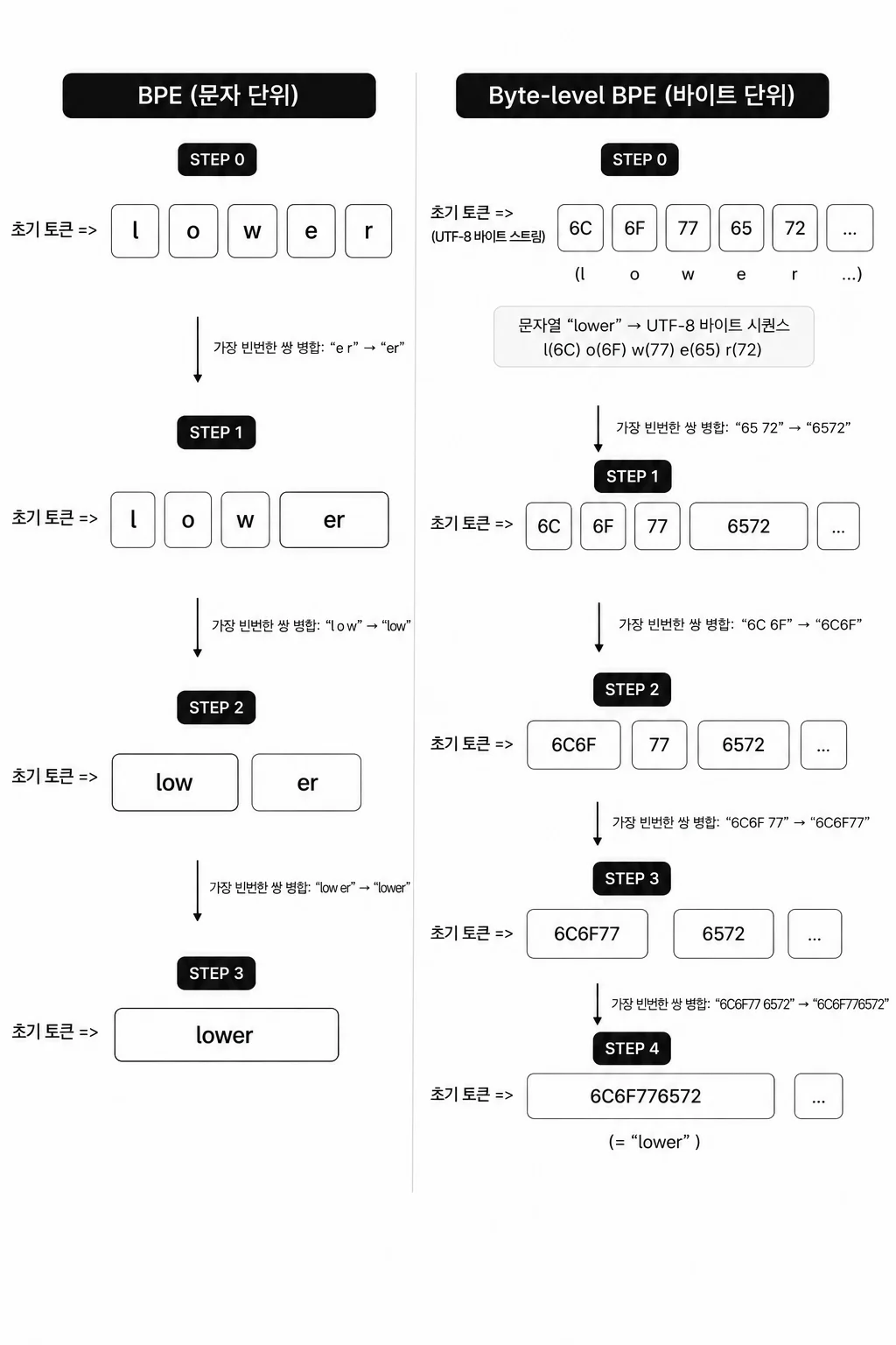
The GPT family takes this one step further with byte-level BPE. It first converts text into a stream of UTF-8 bytes, then applies BPE. This allows the base vocabulary to start with only 256 entries—one for each possible byte—while still being able to encode any text representable in UTF-8 without an unknown token. Whether the input contains emoji, Chinese characters, or special symbols, it is always representable at least at the byte level.

Same Text, Different Token Counts

Because of this structure, the same text can produce very different token counts depending on the tokenizer, the tool that splits human-written text into tokens a model can process. Depending on how its vocabulary was trained, a tokenizer may split the same sentence into finer pieces or larger chunks.

The material OpenAI published alongside GPT-4o illustrates this difference clearly. The o200k_base tokenizer used by the GPT-4o family represents the same text with fewer tokens than cl100k_base, the tokenizer used by the GPT-4 family. It is only about 1.1 times as efficient for English, but the gap widens for other languages. In the short examples OpenAI published, token counts fell by about 1.4 times for Chinese and Japanese, 1.7 times for Korean, and as much as 2.9 times for Hindi. (For Korean users, it is striking how much more noticeable the difference between tokenizer generations is than it is for English users.)

Looking more broadly, there are also disparities between languages themselves. In Yennie Jun's comparison of multiple languages using cl100k_base, English almost always required the fewest tokens for sentences with the same meaning, while languages with their own writing systems tended to require more. Hindi and Bengali could use five times as many tokens as English, and Burmese more than ten times as many. Korean and Chinese also tokenize into more pieces than English, though not as extremely as those languages.

This has an important practical implication. When Anthropic introduced a new tokenizer starting with Opus 4.7, its official pricing documentation stated that the same text could be billed as up to 35% more tokens than with previous models. Even when the per-token rate stays the same, the bill rises in direct proportion to the token count. An honest model comparison therefore has to consider not just the listed rate, but the rate multiplied by the expected number of tokens.

But when these segmented tokens enter the model, they do not go in as literal characters or words. So what form does a token take as model input?

How Tokens Enter the Model

Neural networks cannot work with text directly. Ultimately, a model can compute only with numbers—more precisely, with vectors, which are arrays of numbers. Before entering the model, tokens therefore pass through several stages that convert them into numerical form.

Here is the sequence.

1. Text → tokens: A BPE tokenizer splits the text into token pieces.
2. Token → token ID: Each token maps to an integer ID indicating its place in the vocabulary. For example, if " the" is the 1,234th token in the vocabulary, its ID is 1234.
3. Token ID → embedding vector: The ID selects the corresponding row from the embedding matrix. This matrix is a huge table with dimensions vocabulary size × model dimension (d_model): each token ID corresponds to one row, or one vector. You can think of this vector as a set of coordinates that captures the token's “meaning.”
4. Add positional information: On its own, self-attention has no awareness of token order. In other words, it would view “I like you” and “You I like” as identical. Positional information is therefore injected into each token vector to tell the model the sequence order.

That can feel abstract in words alone, so I have included a widget that lets you interact with all four stages. Change the input sentence or click a token, and you can follow its path from ID to embedding vector, then see positional information added to produce the final input vector. (Only a few dimensions are displayed, but keep in mind that the actual GPT-4 vector has 12,288 dimensions.)

Here, the model dimension (d_model) is the length of the vector used to represent one token. The original Transformer paper used a value of 512, but modern LLMs are much larger. (Even the 7B version of Llama 2 uses 4,096 dimensions.) A larger model dimension can represent subtle differences in token meaning more richly, but it also increases computation and memory requirements.

Methods of injecting positional information have also changed across generations. The original Transformer added position vectors built from sine and cosine functions directly to the embeddings. RoPE (Rotary Position Embedding), now the de facto standard in open LLMs, instead injects relative position during the attention calculation by rotating the Query and Key vectors. (The mechanism differs, but the purpose is the same: giving the Transformer a sense of order.)

In short, the flow is text → tokens → token IDs → embedding vectors (+ positional information) → Transformer input. The “token count” on a bill refers to the second stage of this pipeline: how many tokens the text was split into.

At this point, we know how tokens are created and what form they take when they enter a model. But when the model processes them, why do input and output cost so differently, and how can the cost of sending the same input repeatedly be reduced?

Why Input Is Cheap and Output Is Expensive

Anyone who has worked with tokens has probably wondered about this at some point: on pricing tables, output tokens cost several times more than input tokens. For Anthropic, the output rate is exactly five times the input rate across every model. (Opus is $5 for input and $25 for output, while Haiku is $1 for input and $5 for output.) Why should the same token have a different price depending on whether it is going in or coming out?

The answer is that models process tokens in completely different ways for input and output. LLM inference has two stages.

• prefill (input processing): The model processes all prompt tokens at once and in parallel. Whether the prompt contains 1,000 or 10,000 tokens, the GPU sweeps through them together and calculates the K/V (Key/Value) vectors for each token. The total computation is substantial, but parallel processing makes it efficient per token.
• decode (output generation): The model generates response tokens sequentially, one at a time. After producing one token, it appends that token to the input and generates the next. This repeats until the response is complete.

That asymmetry creates the cost difference. According to Databricks' analysis of inference performance, prefill is a compute-bound stage, while decode is memory-bound. During decode, the model has to read all of its weights from GPU memory again for every token it produces, yet each pass yields exactly one token. Most of the GPU's enormous compute capacity sits idle. (To borrow Databricks' phrasing, you are paying to keep the GPU running without using its available compute.)

In other words, input tokens are processed efficiently together in parallel during prefill, while output tokens must be squeezed out inefficiently one by one. Commercial factors such as demand and margins may also affect pricing, but at the technical level, this decode-stage inefficiency is part of the underlying reason. The principle of “keep outputs short” is therefore more than a generic savings tip: it directly reduces the most expensive stage.

Is there any way to make this inefficient decode stage even slightly less inefficient? This is where KV cache enters the picture.

How Caching Lowers the Price

Prompt caching stores static input in a cache once, then lets subsequent calls read it back at a much lower price. According to Anthropic's official documentation, a cache read costs 0.1 times the base input rate—exactly 10%. A cache write costs 1.25 times the base rate with a five-minute TTL (Time To Live, the period for which the cache remains valid), or twice the base rate with a one-hour TTL. You pay a little extra on the first call, then save 90% from the second call onward.

But how can the price fall by 90%? And why is the requirement that “the prefix must match exactly” so strict? Both answers become clear once we look inside the Transformer.

KV Cache

When processing input tokens, the model creates corresponding Query/Key/Value (Q/K/V) vectors. Self-attention calculates attention scores using the dot product of Query and Key, then uses those scores to produce a weighted sum of the Values. You can think of it as the calculation that determines how much one token should “refer to” every other token.

This is exactly where the decode stage described above becomes a problem. To generate each new token, the model needs the K/V vectors for all preceding tokens. Recalculating them from scratch every time would repeat the same K/V computation endlessly.

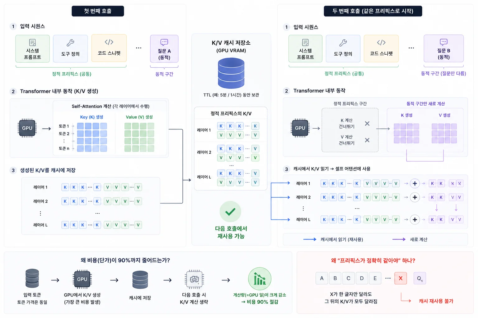
KV cache was introduced to eliminate this duplication. It stores previously calculated K/V vectors, so when generating a new token, the model reads and reuses the preceding tokens' K/V values from the cache instead of calculating them again. Within a single sequence, this reduces the cost of generating one additional token from O(n²), which would recalculate the entire sequence at every step, to O(n), which only requires reading the cache. (Strictly speaking, this describes the cost per step, but the central idea is simple: do not recalculate what has already been computed.) This is also why decode is memory-bound: every step must read the KV cache back from memory.

Reuse Across Calls

If KV cache was originally designed to accelerate decoding within a single response, prompt caching extends the same memory structure beyond one call, reusing it across calls.

The K/V values of a static prefix—such as a system prompt, tool definitions, or code snippets whose beginning remains nearly identical—stay in GPU memory for a five-minute or one-hour TTL. If the next call starts with the same prefix, the model skips that prefix's K/V computation entirely and reads it directly from the cache. More precisely, the input token rate is not reduced by magic: the GPU work required to compute those tokens disappears altogether. The 90% price reduction reflects the computation that has been avoided.

Once you understand this mechanism, the strict requirement that “the prefix must match exactly” also makes sense. A cache hit is determined by whether a cumulative hash of the prefix matches. Because self-attention is causal, changing even one earlier token changes the K/V values of every token that follows. Put just one timestamp at the beginning of a prompt, and its value changes on every call, causing the prefix hash to diverge and invalidating the entire cache after it.

Anthropic reads its cache in the hierarchy tools → system → messages. Changing even one tool definition near the beginning therefore invalidates the whole cache that follows. The conclusion is straightforward: put static content first and dynamic content that changes on every call last if you want the cache to survive.

Caching also has several lesser-known constraints. The minimum cacheable token count differs by model, and even by version within the same family. A prompt shorter than that threshold silently goes uncached even when caching is enabled. (Because these minimum token counts and provider-specific caching policies directly affect cost design, I cover them in detail alongside the pricing tables in the token-saving guide.)

Why the Context Window Sets a Token Limit

The final concept no discussion of tokens can omit is the context window: the maximum number of tokens a model can accept at once. Understanding why this limit exists also clarifies the familiar warning that “longer context costs more.”

The key lies in the computational structure of self-attention. Attention involves every token referring to every other token once. With n tokens, there are n × n token pairs, so the computation and memory required by self-attention grow with the square of the sequence length n. Double the number of tokens, and the attention cost quadruples. (It is worth clarifying that the entire model is not O(n²); the attention stage is.)

Hugging Face's estimates show just how steep this quadratic growth becomes. With standard, unoptimized attention, storing the attention score matrix alone requires only about 50 MB for an input of 1,000 tokens, but about 19 GB for 16,000 tokens and nearly 1 TB for 100,000 tokens.

The KV cache described earlier also consumes memory in proportion to the number of tokens. As the context grows, the K/V values the model must retain accumulate linearly. In the end, the context-window limit is a boundary set by physical constraints: beyond that point, the memory and computation become unmanageable.

This is why carrying a long conversation forward unchanged is not simply a matter of adding more input tokens. Attention costs grow quadratically, and as the token count approaches the limit, the model's ability to handle information accurately also declines. (This loss of accuracy is directly related to context rot, which I discuss in the token-saving guide. It is precisely why keeping context lean benefits both cost and answer quality.)

Conclusion

Putting it all together, the way tokens work comes down to a few simple facts. A token is a vocabulary unit created by BPE from frequently used patterns, and it enters the model as an embedding vector after being mapped to a token ID. Input is processed all at once through parallel prefill, while output is more expensive because it must be squeezed out one token at a time, and the KV cache reduces that inefficiency by reusing K/V values. Caching lowers the price not through magic, but because the Transformer does not recalculate K/V values it has already computed, and the demanding requirement for an exact prefix follows directly from this architecture. Finally, longer context costs more because attention cost grows with the square of the token count.

Once you understand this foundation, the economics become much clearer. Strategies such as shortening output, arranging prompts so the cache remains intact, keeping context lean, and switching to a cheaper model when it gives the same answer all rest on these principles. If you have read this far because you wanted to understand the mechanics, I recommend continuing with the token-saving guide to see how these principles translate into real cost reductions.

참고 자료

Philip Gage, A New Algorithm for Data Compression (1994)

Sennrich, Haddow, Birch, Neural Machine Translation of Rare Words with Subword Units (ACL 2016)

Jay Alammar, The Illustrated Transformer

HuggingFace, Byte-Pair Encoding tokenization

HuggingFace, Transformers KV Cache strategies

OpenAI, tiktoken

OpenAI, Hello GPT-4o (Language tokenization)

Yennie Jun, All languages are NOT created (tokenized) equal

Databricks, LLM Inference Performance Engineering Best Practices

Baseten, A guide to LLM inference and performance

Anthropic, Prompt Caching